Biosignals: sources, propagation, acquisition, processing

Dr Germano Gallicchio

Lecturer in Psychophysiology and Cognitive Neuroscience

School of Psychology and Sport Science, Bangor University, UK

profile | research | software | learning resources | book meeting

On a computer press F11 to de/activate full-screen view.

For smartphone and review: Bottom left menu -> Tools -> PDF Export Mode.

For pdf document: use “learning resources” link above.

Last modified: 2026-02-16

QR code to
these slides:

PIN

0000

Objectives:

By the end of this session, you should be able to elaborate on:

Approach:

• a mixture of concepts and intuition
• questions welcome at any time. Feel free to contact me.

Content

1. Principles of biosignals propagation
2. Acquisition
   • The recording chain
3. Biosignals processing

Concepts and intuitions.

Source and propagation: the ripple analogy

[Biosignals] are complex ramifications of the [electrochemical] spread of action [and graded] potentials in a conductive medium, the human body.

– Adapted from Stern et al. 2001

The ripple analogy: a stone (source) is thrown in a water body (medium) creating a ripple (propagation)

ANALOGY	MEANING
stone	electrochemical event
water	medium for propagation
ripple	electrical field

Stern, R. M., Ray, W. J., & Quigley, K. S. (2001). Psychophysiological recording. Oxford University Press, USA.

Some basic principles of biosignals propagation:

We will discuss the following principles of biosignals propagation:

Principles of biosignals propagation > Volume conduction

• Electrical fields spread through biological tissue via ionic currents in the extracellular fluid
• Propagation is rapid but not instantaneous (limited by tissue resistance and capacitance)
• Propagation medium: extracellular fluid
• Volume conduction is good: it allows to detect the phenomenon at a distance
• Volume conduction is bad: multiple sources get mixed

Principles of biosignals propagation > Spatial degradation

• The signal propagates through a medium that is an imperfect conductor, so it degrades as it propagates
• The electrical field is stronger near its source
• Its magnitude diminishes gradually the farther from the source

Principles of biosignals propagation > Impedance

• Resistance to propagation of the electrical field
• Mainly due to the outer layer of the skin, which has low water/ion content, so it’s a poor conductor.
• It can be decreased through mild skin abrasion

Principles of biosignals propagation > Orientation

• Each electrical event has a geometry: a dipole
• Just like vectors, multiple dipoles have a resultant
• Dipoles in the same orientation summate and their resultant is larger than the individual dipoles
• Dipoles in the opposite orientation cancel out and their resultant is smaller than the individual dipoles (or even null)
• Not all dipoles’ resultants are big enough to be detectable from the skin

Principles of biosignals propagation > Summation

• Most electro-chemical events are very small and involve few cells
• Because of their small magnitude and of spatial degradation, in principle we cannot detect them from the skin
• However… small electro-chemical potentials can summate into a larger potential when the dipoles occur:
  • at the same time
  • in the same area
  • with roughly the same orientation

Acquisition

Overarching objective:

• Measure the electrical field associated with the biological event (the signal)

• While discarding as much as possible of other, biological or not, events (the noise)

• maximize signal to noise ratio:

\[ SNR = \frac{S}{N} \]

Signal to Noise Ratio (SNR) is a measure of how much the signal stands out from the noise. The higher the SNR, the better the quality of the recording.

Acquisition > The recording chain:

The recording chain consists of the following stages:

Sensors > Electrodes

• Conductive material

• Used in pairs to measure a difference in voltage. Note: One electrode alone cannot measure anything

• At the interface between electrode and skin, electro-chemical reactions occur consisting of exchange of ions.

• The exchange of ion generates an unwanted voltage, called offset potential (or bias potential).

• The offset potential is a source of noise that can interfere with the signal. It can be reduced by using certain types of electrodes and by preparing the skin properly.

• Desirable property of electrodes: stability against offset potential

Sensors > Electrodes > metals

Factors affecting electrode stability:

• temperature
• electrolyte composition (between the electrode and the skin)
• metal type (the electrode)

Lykken (1959) experimented with different metals.

Left pairs of electrode of various metals in a saline solution (electrolyte) for 1 hour.

Among several metals such as platinum, zinc, silver, silver / silver chloride (Ag/AgCl) showed the lowest offset potential. To this day, mostly electrodes are made of this metal.

Ag/AgCl = “chlorided silver” or “silver / silver chloride” meaning silver coated with silver chloride.

Lykken, D. T. (1959). Properties of electrode used in electrodermal measurement. Journal of Comparative and Physiological Psychology, 52(5), 629.

Sensors > Electrodes > electrode-skin impedance

Desirable property of skin-electrode interface low impedance, so the signal passes through with little resistance.

skin –> electrolytic gel –> electrode

Skin preparation to lower impedance:

• mild abrasion with sandpaper or abrasive paste (scrub) to remove outer layer of skin
• alcohol to clean residuals and to degrease the skin
• More abrasion –> lower impedance (but also more discomfort and risk of skin damage. So, a balance is needed.)

Impedance matters more for smaller signals (e.g., EEG) because they are more affected by noise. For larger signals (e.g., ECG), impedance matters less because the signal is stronger and can stand out from the noise even with higher impedance.

Sensors > Electrodes > Types

1. Disposable passive electrodes:

• pregelled (ready to use)
• low cost, but not reusable
• search “pre-gelled electrode” for an example of disposable electrode

2. Passive electrodes:

• require gel and cleaning (requires care)
• reusable
• search “cup electrode” for an example of passive electrode

3. Active electrodes:

• like n.2 but with pre-amplifier (requires extra care)
• more expensive but more stable (lower offset potential) because the pre-amplifier enhances the signal before it is affected by noise
• search “BioSemi active electrode” for an example of active electrode

Sensors > Transducers

While biological events have electrical nature, certain electrical fields are difficult to detect. Non-electrical consequences of these events are easier to detect.

Transducers convert (transduce) non-electrical signals to electrical signals (for the next steps of the recording chain)

For example, changes in blood volume or pupil diameter are easier to detect than the electrical field generated by the underlying electro-chemical event.

Sensors > Transducers > example: changes in blood volume

Photo-conductive transducer:

• infra-red (IR) light is sent from a light emitter
• IR-light passes through certain biological tissues (e.g., skin) but it is reflected back by other tissues (e.g., blood)
• By measuring the difference between IR-light emitted and received back, we can infer blood volume
• commonly placed on finger or earlobe

A common application: photoplethysmography (PPG) applied to the finger or earlobe, and used to measure heart rate (HR) and heart rate variability (HRV) by detecting the changes in blood volume that occur with each heartbeat.

Sensors > Transducers > example: changes in pupil diameter

Photo-sensitive transducer:

• infra-red (IR) light is sent from a light emitter
• IR-light is reflected differently by pupil and iris
• By measuring the areas with more and less IR-light reflection, we can infer the size of the diameter

A common application: pupillometry, which is the measurement of pupil diameter. Changes in pupil diameter can be indicative of cognitive and emotional processes, as well as arousal levels.

Signal Conditioner

Modern signal conditioners carry out multiple functions. The two main functions are:

• Filtering: removes unwanted frequencies (more on this below)
• Amplification: multiplies the filtered signal by a gain factor

Historical note: Older systems used a separate “coupler” component between sensors and signal conditioner. Modern systems integrate these functions directly into the signal conditioner.

Signal Conditioner > Filtering

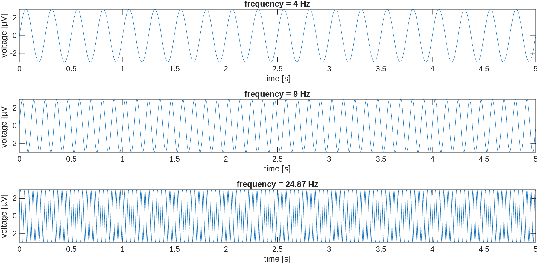
Let’s first see waveforms of different frequencies.

waves of different frequency

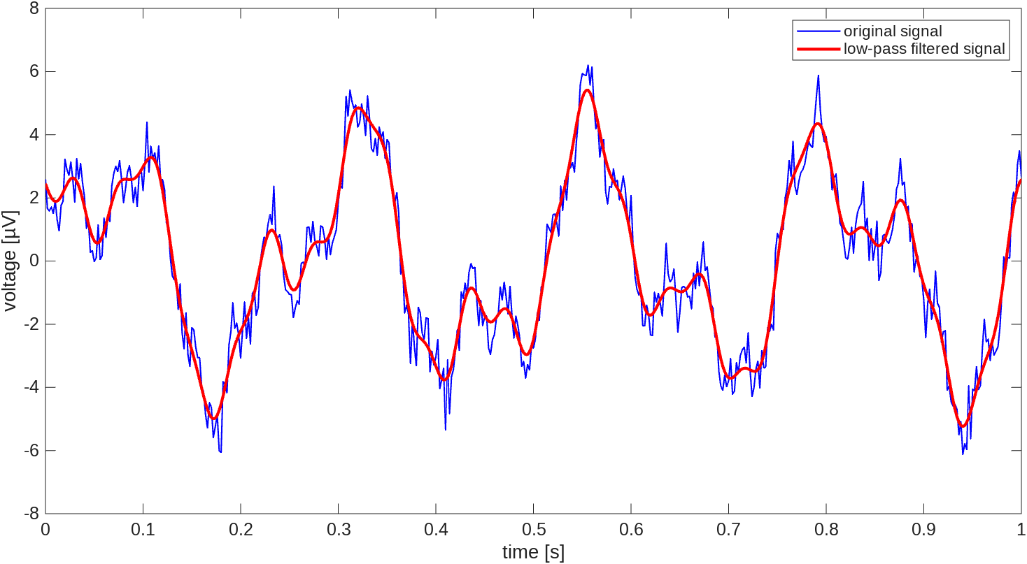
Filtering is the process of removing unwanted frequencies from the signal. Basic filter types:

• low-pass
• high-pass
• band-pass
• notch

Signal Conditioner > Filtering > Low-pass

Filters out fast (high) frequencies and therefore retains slow (low) frequencies

low-pass filtering

Also called “high-cut” filter, but less frequently.

Signal Conditioner > Filtering > High-pass

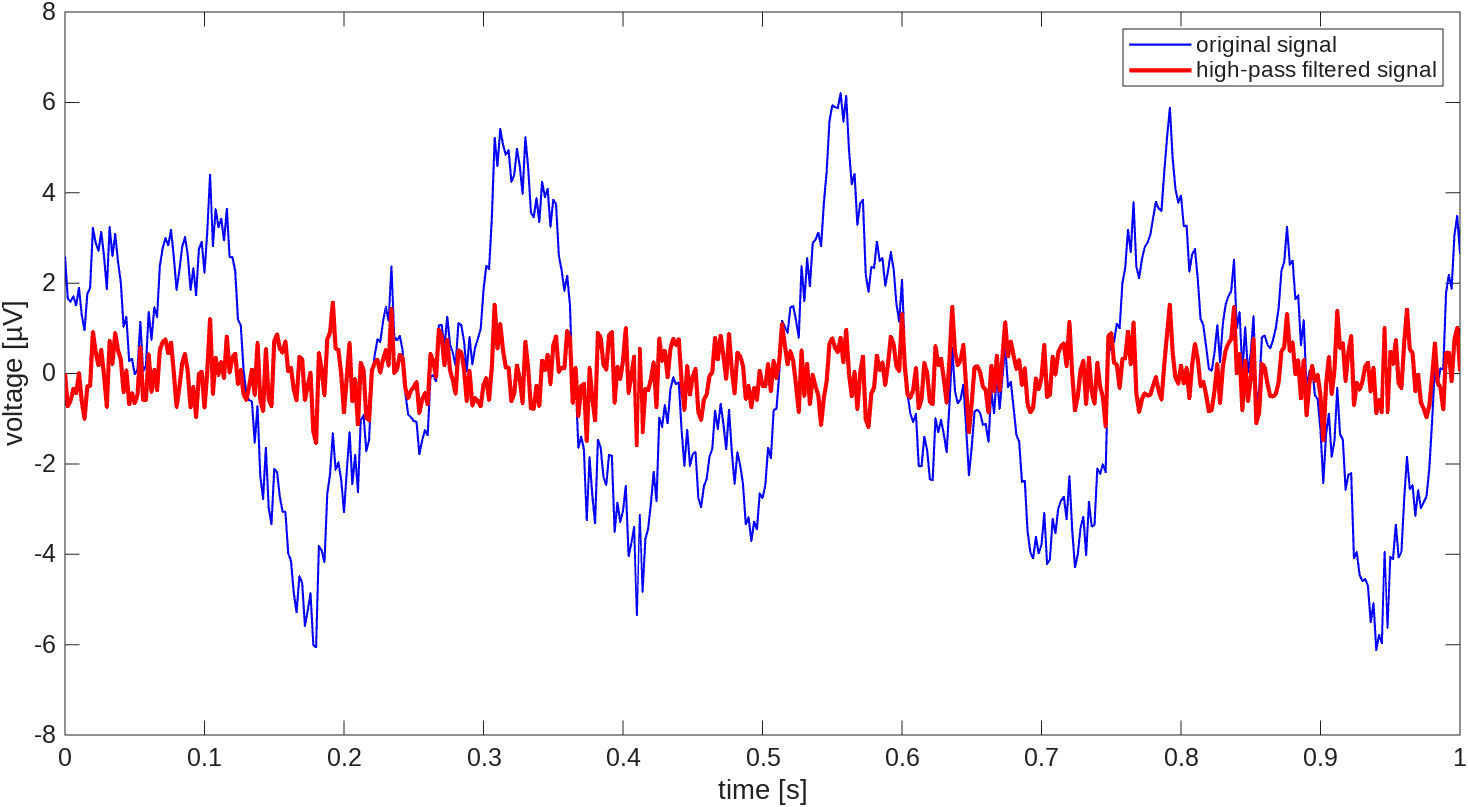
Filters out slow (low) frequencies and therefore retains fast (high) frequencies

high-pass filtering

Also called “low-cut” filter, but less frequently.

Signal Conditioner > Filtering > Band-pass

A combination of high-pass and low-pass filters to allow frequencies between two cut-off values, which describe a frequency band. Frequencies outside of this band are filtered out.

Signal Conditioner > Filtering > Notch

Filters out only one frequency (and those immediately near it). Just like a very narrow band-stop filter.

Used to minimize the electrical interference from mains electricity (alternating current). In the UK, it is 50 Hz.

Signal Conditioner > Filtering > Filter parameters

Filters require:

• cut-off frequency value(s)
• other parameters having to do with how sharp the transition is from filtered frequencies to non-filtered frequencies

Depending on the sharpness parameter, frequencies near the transition are partly retained

In theory, a filter with a sharp transition is better. In practice, too sharp will create distortions.

Signal Conditioner > Amplification

Signals of interest are often very small in magnitude (e.g., microvolts for EEG) and can be easily obscured by noise. Amplification is used to increase the magnitude of the signal to make it more distinguishable from noise.

The multiplication factor by which the signal is amplified is called gain.

Traditionally, the signal is amplified so its magnitude reaches approximately 1 V.

For example, a signal with magnitude 1 mV will be multiplied by 1000 to reach 1 V. (In this example, the gain is 1000.)

Note: Important to amplify the signal but not the noise. That’s why filtering happens before amplifying (with some exceptions)

Analog-to-digital conversion (ADC) > Digitization

sampling a waveform

The signal acquired by the sensors and processed by the signal conditioner is an analog signal.

A continuous signal that can take any value within a certain range.

Example: Imagine an uninterrupted line on a polygraph.

The signal that the computer can store must be digital.

A digital signal is discrete (i.e., not continuous) and can only take certain values at specific time points.

Example: imagine a series of dots on a polygraph, where each dot represents a sample of the signal at a specific time point.

Analog-to-digital conversion (ADC) > Digitization > Sampling rate and bit depth

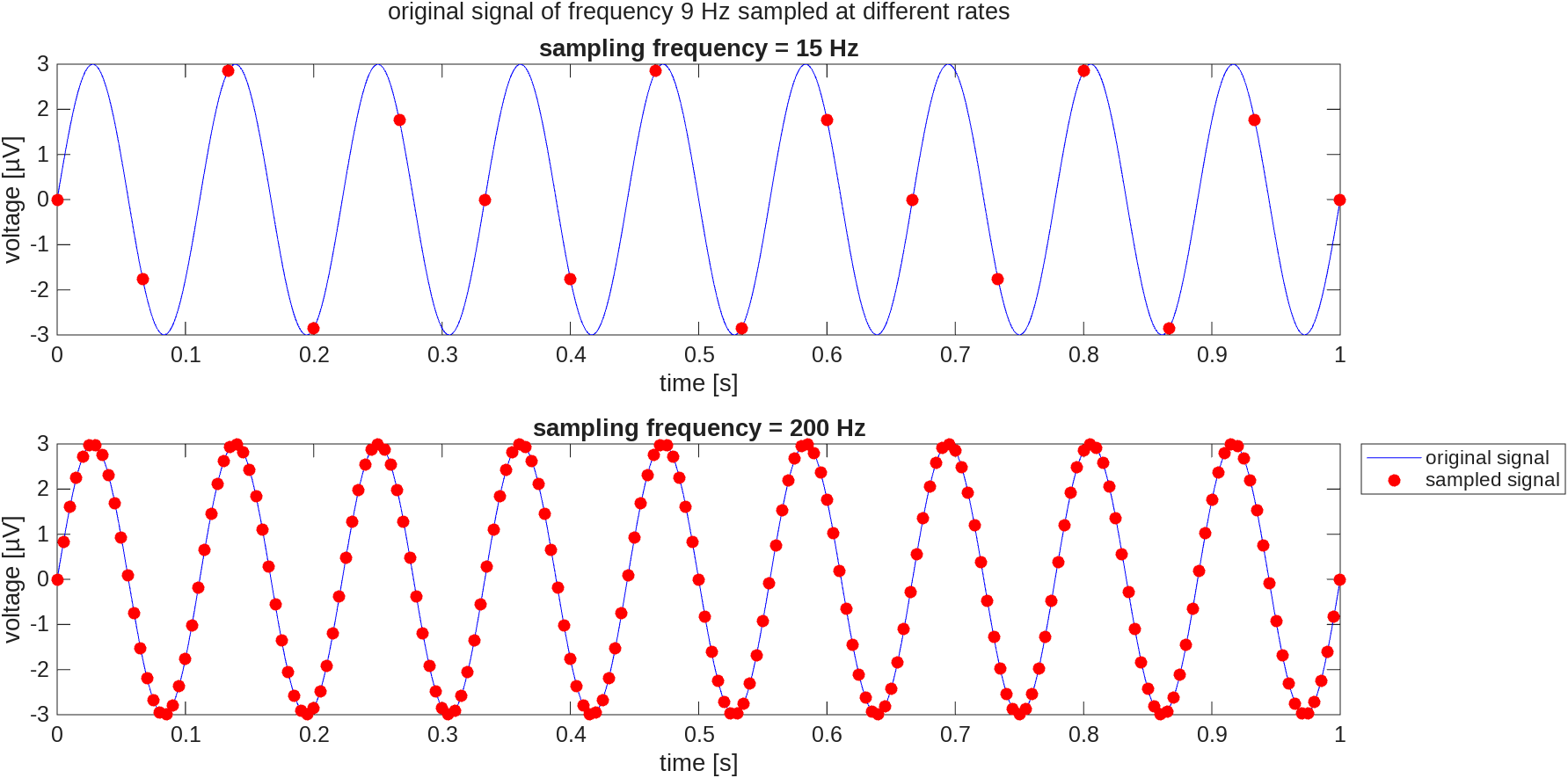
Digitization (or discretization) involves taking a series of samples of the analog (or continuous) signal, every so often–that is, at a certain sampling rate–and assigning a value to each sample–bit depth.

Sampling rate: how many samples are taken in a unit of time. For example, 10 Hz means 10 samples per second, 0.5 Hz means 0.5 samples per second (i.e., 1 sample every 2 seconds).

Bit depth: how many values can be assigned to each sample (e.g., 8-bit means 256 values, 16-bit means 65536 values). For example, if the signal can range from -100 to 100 microvolts, an 8-bit system would assign a value to each sample in increments of approximately 0.78 microvolts (200/256), while a 16-bit system would assign a value in increments of approximately 0.003 microvolts (200/65536).

Analog-to-digital conversion (ADC) > Digitization > Quality

The digitized signal is an approximation of the original analog signal. The quality of the approximation depends on how often we take samples of the analog signal (sampling rate) and how many values we can assign to each sample (bit depth).

• Greater sampling rate –> better approximation, but more digital storage/memory is required.
• Greater bit depth –> better approximation, but more digital storage/memory is required.

Examples:

1. You are watching a video of a football game and want to take screenshots to capture the action. How often should you take the screenshots (sampling rate)? How many different colors should you use in the screenshots (bit depth)?

2. You are watching the clouds in the sky and want to take photos to capture their movement. How often should you take the photos (sampling rate)? How many different colors should you use in the photos (bit depth)?

Most likely, you would take screenshots more frequently and use more colors for the football game than for the clouds, because the football game has more rapid and complex changes that require a higher sampling rate and bit depth to capture accurately.

Too high sampling: you might end up with a lot of redundant information that takes up storage space and makes it harder to analyze the data.

Too low sampling: you might miss important moments in the football game (e.g., a goal) or the movement of the clouds (e.g., a sudden change in direction). Distortion due to undersampling is called aliasing.

To avoid aliasing, the sampling rate should be at least 2-5 times larger than the larger frequency contained in the signal.

Biosignals processing > Signal reduction

Signal reduction. Term indicating the signal processing happening before statistics are run. For example:

• Reduce the complex ECG waveform into a simpler series of heart rate (HR) values
• Reduce the complex EOG waveform into a simpler number of eye blinks within a minute

Signal reduction can happen:

• Online (during the acquisition stage, in real time)
• Offline (after the acquisition stage)

Biosignal processing > Temporal dynamics

The temporal dynamics of biological activity can be classified as:

Tonic activity

• Background level over a relatively long period of time
• Useful for studying the signal “on average”
• Generally recorded at rest, but it could be recorded during a relatively long activity
• Sometimes interesting as a baseline for phasic activity (next slide); sometimes interesting by itself (e.g., essential hypertension)

Phasic activity

• Transient activity over a relatively short period of time
• Useful for studying the short-lived fluctuations on top of tonic activity
• Generally specific to reaction to certain events (e.g., a stimulus is presented that needs processing, an action is performed)
• Can be a change in amplitude of the signal, frequency of the signal, or other (more complex) parameters

Change scores Typical use: describe transient changes (phasic activity) from baseline (tonic activity)

Notable types of change scores:

• Subtraction: \(A - B\)
• Percentage change: \(\frac{A-B}{B} \times 100\)
• Decibel change: \(10 \log_{10}\frac{A}{B}\)

(A = activity; B = baseline)

Biosignals processing > Time vs frequency domain

Time domain. Features that develop over time. For example:

• Durations (e.g., eye blink duration)
• Rate (e.g., number of ECG R-waves in 1 minute)
• Amplitude (e.g., max blood pressure)
• Latency (e.g., time between stimulus presentation and peak of a certain EEG component)

Frequency (spectral) domain. Features linked to oscillatory trends. For example:

• The magnitude of oscillations at certain frequencies
• The positioning of oscillations at certain frequencies
• The coherence of oscillations at certain frequencies (see next slide)

Caveats with the acquisition and processing of each specific biological signal of psychological interest.