In classical measurement theory, every observed score is the sum of two components:
true score
error
In the Week 1 task, the true score is the speed with which a participant’s nervous system responds to a visual stimulus.
Sources of error in the class data:
display refresh (approximately 17 ms per frame at 60 Hz)
touchscreen and input latency
momentary lapses of attention, blinks, distraction
in Week 2, the timer’s own reaction time at the start and end of each run
Error: random and systematic
Random error (aka, noise)
Varies unpredictably in magnitude and direction from one observation to the next.
a slow trial following a blink
a stopwatch started slightly early and stopped slightly late
Reduced by averaging across observations.
Systematic error (aka, bias)
Displaces observations consistently in one direction.
the input latency of a particular device
web-based tasks recording longer times than laboratory equipment
Not reduced by averaging; requires a change in the measurement procedure.
Averaging across trials
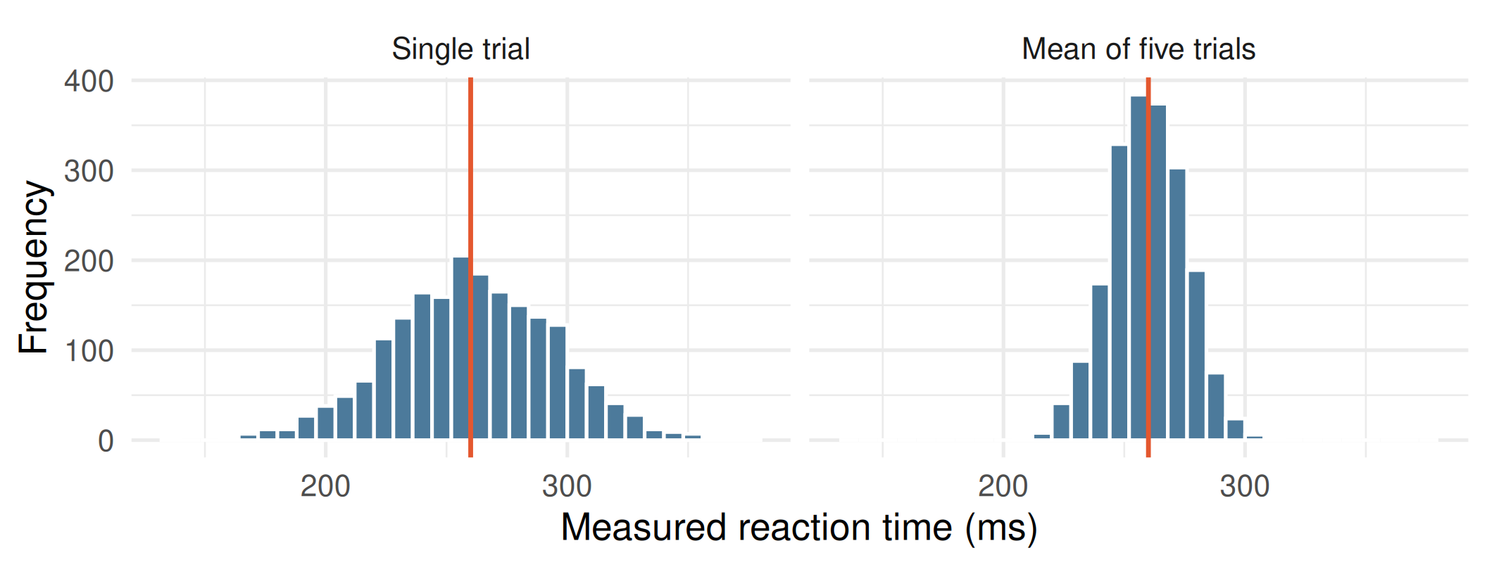
Simulated data: one participant with a true reaction time of 260 ms (red line), measured 2000 times.
The mean of several trials is a more precise estimate of the true score than any single trial, because random errors partially cancel.
Best trial versus mean performance
The fastest trial is the observation in which random error happened to favour the participant most.
The mean of all trials allows positive and negative errors to offset one another.
For describing a participant’s typical performance, the mean (or median) of all trials is preferred to the single best trial.
Reliability and validity
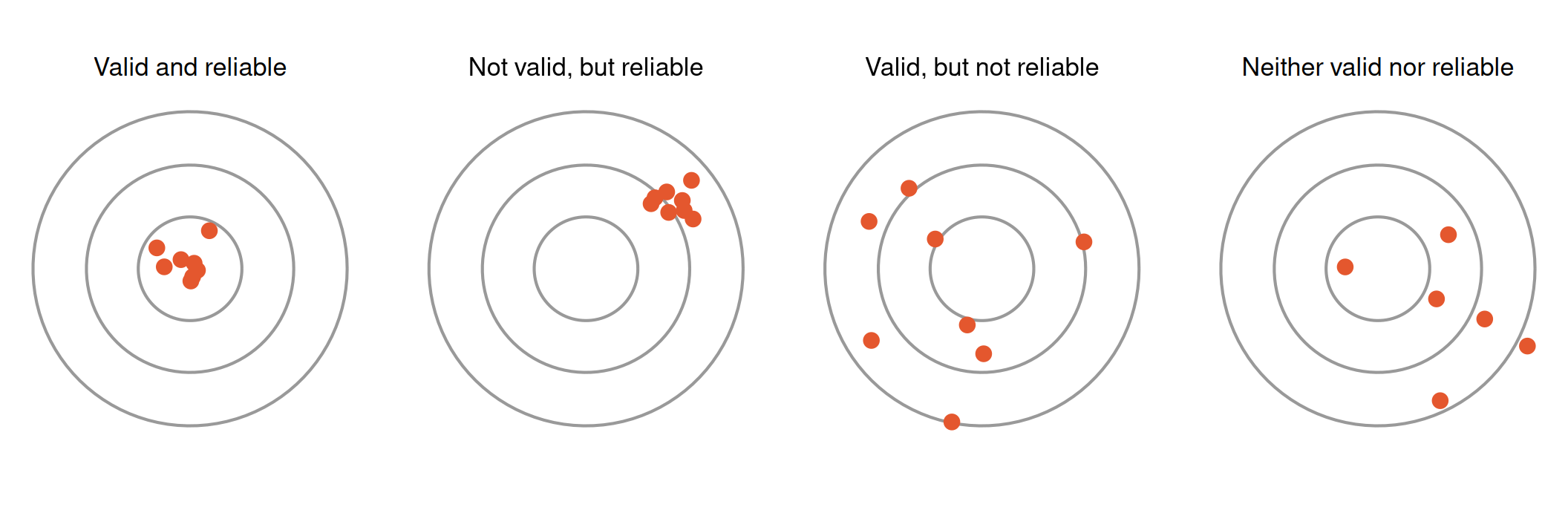
Reliability: the consistency of a measure across repeated observations.
Validity: the extent to which a measure reflects the construct it is intended to measure. In this illustration, measurements centred on the target are valid (unbiased on average).
Test–retest reliability
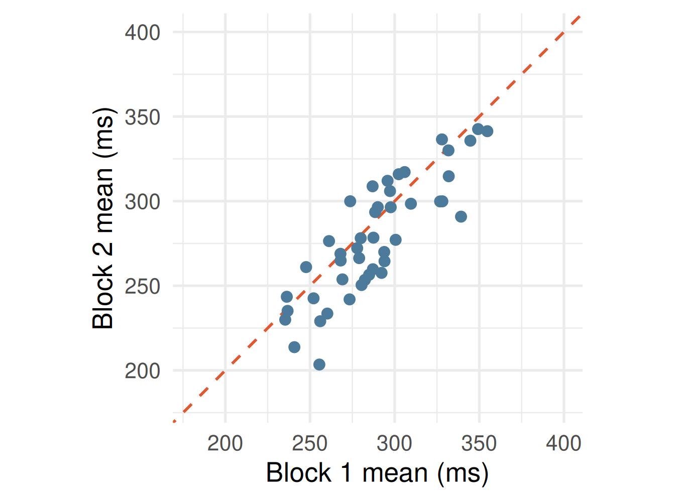
Simulated data. Points on the dashed line indicate identical scores in both blocks; the closer the points lie to the line, the higher the test–retest reliability.
Validity of device-based measures
Simple visual reaction time measured with laboratory equipment is typically in the region of 200–250 ms.
The class means, obtained on personal devices, were slightly higher.
Scores differed systematically between smartphones and laptops.
The same participant would therefore obtain different scores on different devices.
A measure can be highly reliable and nonetheless biased.
The Week 1 score is a valid measure of performance on a particular device; it is a less valid measure of nervous-system processing speed.
Distributions
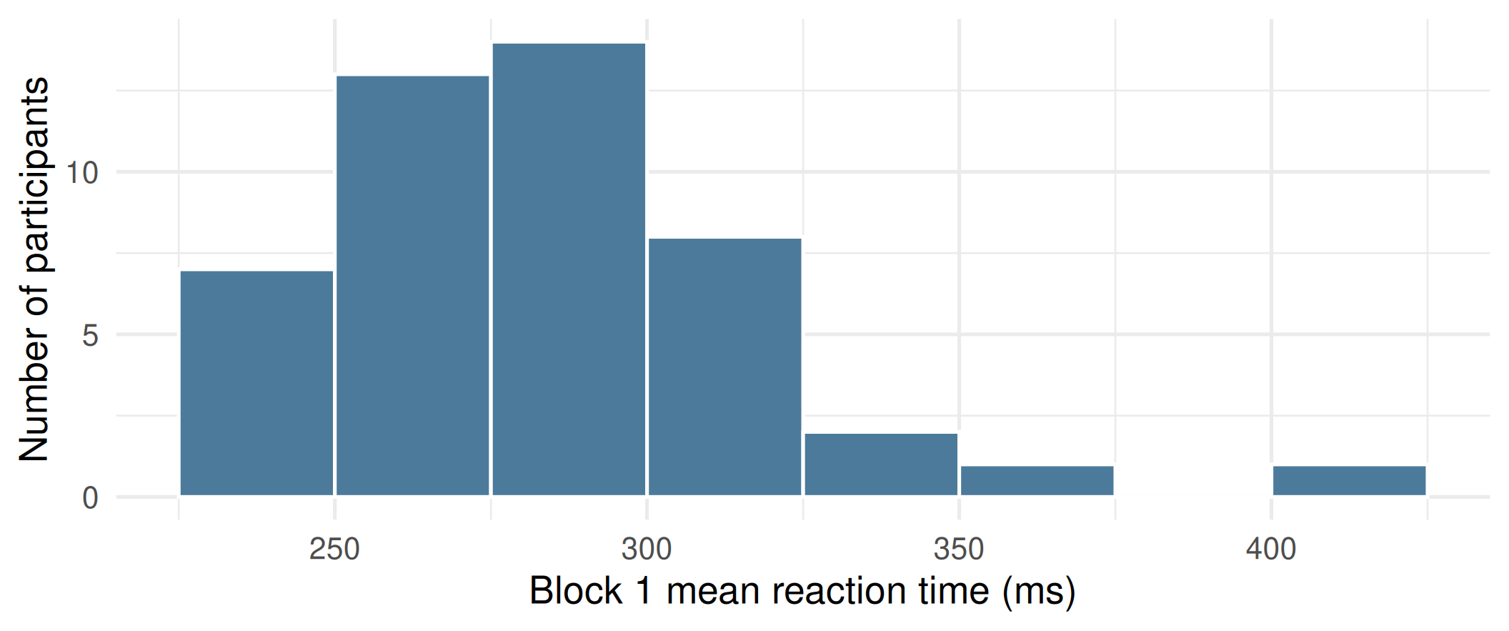
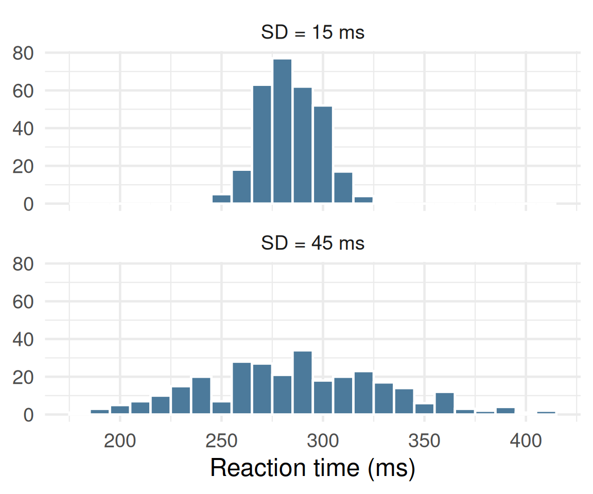
A histogram shows the number of observations falling within each interval (here, 25 ms).
Three properties are of interest: central tendency, dispersion, and shape.
Measures of central tendency
Mean: the sum of all observations divided by their number.
Median: the middle value when observations are ranked in order.
In a symmetric distribution the two coincide.
Five observations: 240, 260, 270, 280, 300 ms
mean = 270
median = 270
One extreme observation: 240, 260, 270, 280, 900 ms
mean = 390
median = 270
The mean is sensitive to extreme values; the median is robust to them.
Measures of dispersion
Range: the difference between the largest and smallest observations.
Determined entirely by the two most extreme observations.
Standard deviation (SD): approximately, the typical distance of an observation from the mean.
Determined by every observation.
Two distributions with the same mean may differ substantially in dispersion. A measure of central tendency should therefore be reported together with a measure of dispersion.
Within-participant difference scores
Participants differ considerably from one another (between-participant variability).
To assess the effect of a change in conditions, each participant can be compared with themselves.
Participant
Block 1
Block 2
Difference (2 − 1)
A
312
298
−14
B
251
249
−2
C
290
301
+11
A negative difference indicates a faster response in block 2. The mean difference estimates the average change, with stable differences between participants removed.
Within-participant comparisons in this module
Week
Conditions compared within each participant
Difference score
2
auditory vs visual signal
visual − auditory
5
valid vs invalid spatial cue
invalid − valid
7
congruent vs incongruent Stroop trials
incongruent − congruent
11
two vs eight response alternatives
eight − two
Each of these practicals yields one difference score per participant.
Bar plot, data points and error bars
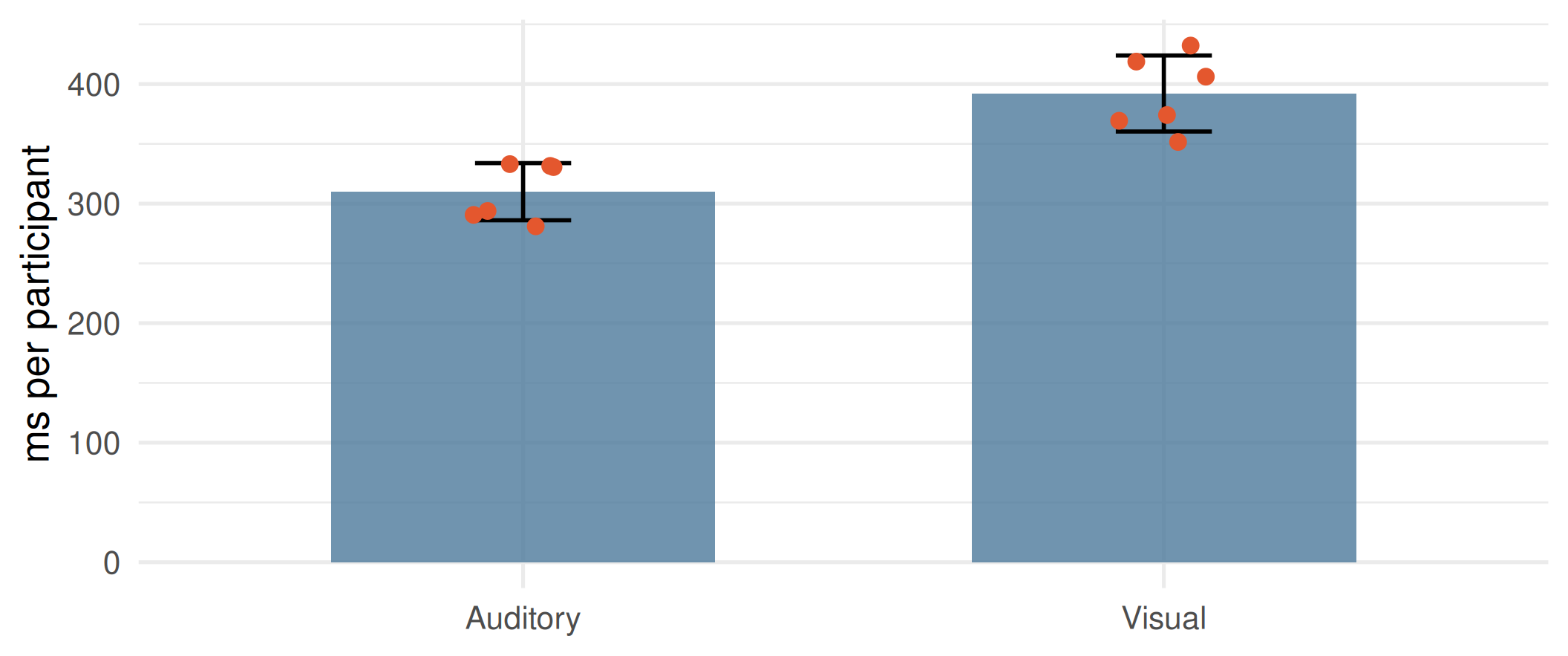
Bar height: mean. Error bar: here, ±1 SD. Points: individual observations.
Error bars may represent the SD, the standard error, or a confidence interval. The figure caption must state which.
Axis truncation
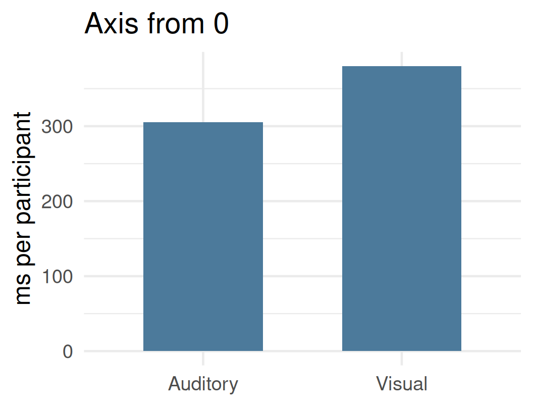
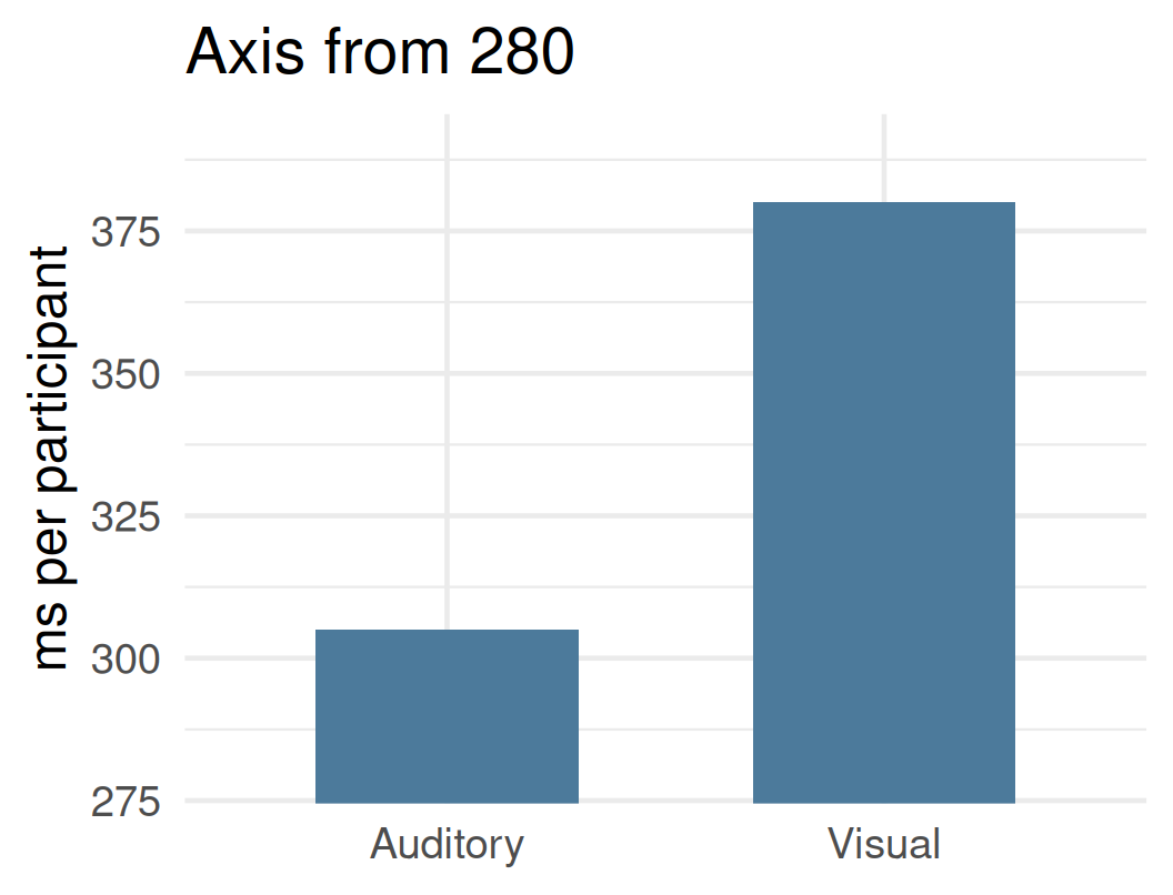
Identical values. In the right-hand panel the visual condition appears approximately four times slower; the true difference is approximately 25%.
Bar length represents magnitude, so bar charts should begin at zero. Where an axis is truncated, this should be evident and justified.
Evaluating a figure
Which variable was measured, and in which units?
What does each graphical element represent: an individual observation, a group mean, or a count?
Which conditions or groups are being compared?
Where does each axis begin, and what do the error bars represent?
These questions will be applied to a published article in Week 6, on which the coursework is based.
Review questions
Identify one source of random error and one source of systematic error in the Week 1 and Week 2 data.
Explain why the mean of five trials provides a better estimate of a participant’s reaction time than the fastest trial.
In a sample of ten, one large observation is 900 ms. Which is affected more, the mean or the median, and why?
What is the advantage of comparing each participant with themselves rather than comparing two separate groups?
Review (MCQs 1)
A reaction-time task administered on a smartphone consistently records times approximately 30 ms longer than laboratory equipment. This is an example of:
random error
systematic error
a reliable and valid measure
a difference score
correct answer: B
Review (MCQs 2)
A participant’s mean reaction times in two blocks are almost identical. This primarily indicates that the measure is:
valid
reliable
unbiased
accurate
correct answer: B
Review (MCQs 3)
Reaction times of 250, 260, 270, 280 and 1000 ms are recorded. Which statement is correct?
The mean and the median are equal
The median is greater than the mean
The mean is greater than the median
The standard deviation is zero
correct answer: C
Review (MCQs 4)
Two groups have the same mean reaction time, but group A has a substantially larger standard deviation. This indicates that:
group A responded faster
participants in group A differ more from one another
group A contains more participants
the measurements in group A are invalid
correct answer: B
Review (MCQs 5)
The y-axis of a bar chart begins at 280 ms rather than at zero. The principal risk is that:
the means are calculated incorrectly
the error bars are omitted
the difference between conditions appears larger than it is
the units of measurement change
correct answer: C
Review (MCQs 6)
Each participant is tested with and without a distractor, and a difference score (with − without) is computed for each participant. The principal advantage of this approach is that:
only one participant is required
stable differences between participants are removed from the comparison
the validity of the measure is guaranteed
the mean becomes equal to the median
correct answer: B
Next session
Perception. Please note the change of day and time: Friday 23 October, 15:00–18:00.
The session begins with the practical. Participants will provide perceptual estimates, and the class data will be examined in the lecture that follows.
Today’s practical: analysis of the class data in Excel for the web. No installation is required.
Optional: standard deviation and standard error
The SD describes the variability of individual observations around the mean.
The standard error (SE) describes the variability of the sample mean across hypothetical repeated samples of the same size.
SE = SD ÷ √n. As sample size increases, the SE decreases, whereas the SD remains approximately constant.
Published figures frequently display SE bars, which describe the precision of the mean rather than the variability of participants.
Optional: distinguishing a difference from noise
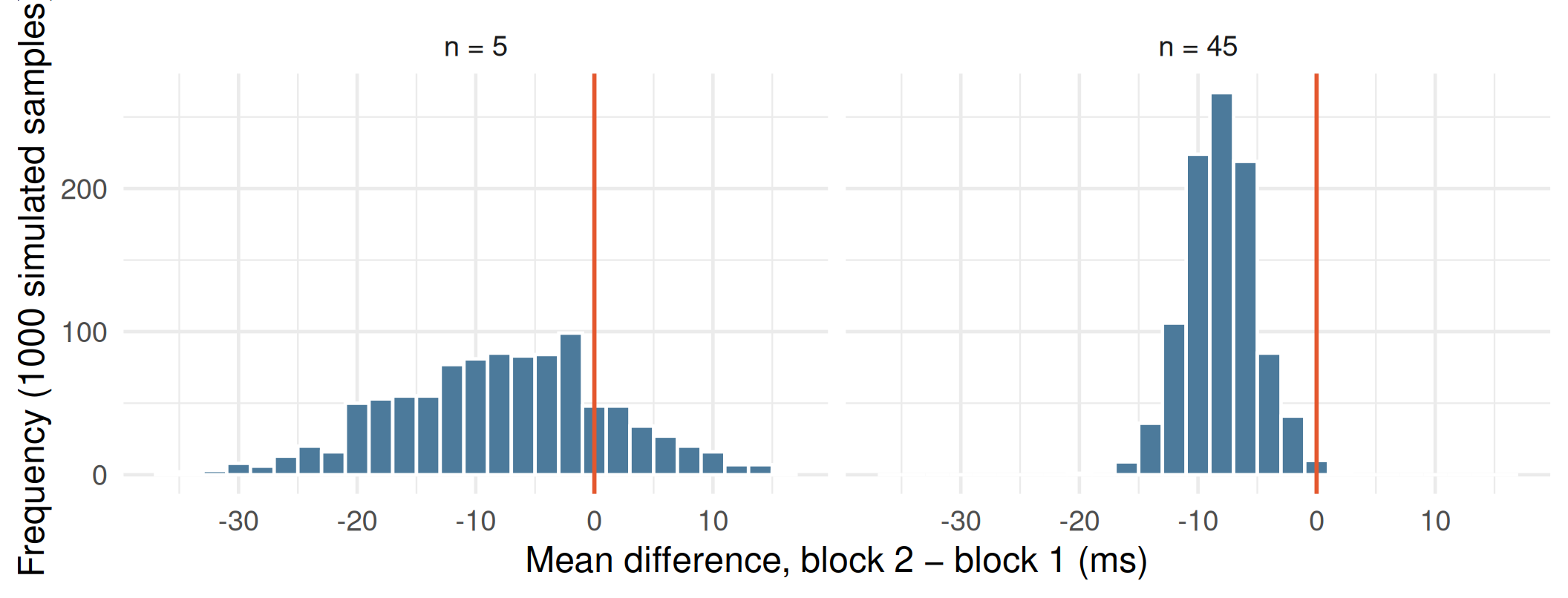
Simulated data: a true improvement of 8 ms with individual variability of 20 ms. With five participants, a substantial proportion of samples show no improvement or a slowing; with 45 participants, very few do.
A difference is more convincing when it is large relative to the variability and is observed across a sufficient number of participants. Inferential statistics formalise this reasoning.
Optional: skewness
Reaction-time distributions are typically positively skewed: responses cannot be much faster than approximately 150 ms, but can be considerably slower (e.g., following a lapse of attention).
In a positively skewed distribution the mean exceeds the median.
For this reason, reaction-time studies frequently summarise each participant’s performance with the median.